5. Hits and effects

This page asks which treatments moved away from the controls, and which measurements changed. Both answers come with a p-value from a permutation null, and both are computed on the same object.

import matplotlib.pyplot as plt
import numpy as np

import mantispy as mt

A plate with known answers

synthetic_plate injects a known effect into known features, so every result on this page can be checked against uns["mantispy"]["truth"].

cells = mt.ds.synthetic_plate(n_wells=192, n_cells=40, n_features=25, n_perturbations=3, effect_size=3.0, seed=0)
mt.pp.normalize(cells, by="Metadata_Plate", reference="negcon")
wells = mt.tl.aggregate(cells, min_cells=0)
wells

AnnData object with n_obs × n_vars = 192 × 25
    obs: 'Metadata_Plate', 'Metadata_Well', 'Metadata_CellCount', 'Metadata_Row', 'Metadata_Col', 'Metadata_Perturbation', 'Metadata_Control', 'Metadata_Batch', 'Metadata_ImageNumber'
    var: 'object', 'feature_group', 'feature', 'channel', 'scale', 'angle', 'gray_levels', 'radial_bin', 'params', 'is_feature', 'degenerate_scale'
    uns: 'mantispy'
    layers: None (.X)

Calling hits

tl.hit_calling measures how far each group sits from the controls and compares that with a null built by drawing groups of the same size from the control wells. The question is whether this group is further out than the same number of control wells would be.

Drawing the null from all rows would put the real hits into the null, and a screen where half the compounds work would look like one where none do.

A permutation p-value is never zero. With 1000 permutations the smallest possible value is 1/1001, and anything smaller would claim more resolution than the permutations provide.

mt.tl.hit_calling(wells, n_permutations=1000)
wells.uns["mantispy"]["hits"].round(4)

	group	n_obs	distance	pvalue	qvalue	is_hit
0	DMSO	48	55.5582	1.000	1.0000	False
1	pert00	48	3086.7268	0.001	0.0013	True
2	pert01	48	1521.9842	0.001	0.0013	True
3	pert02	48	2204.6422	0.001	0.0013	True

ax = mt.pl.hits(wells)
plt.show()

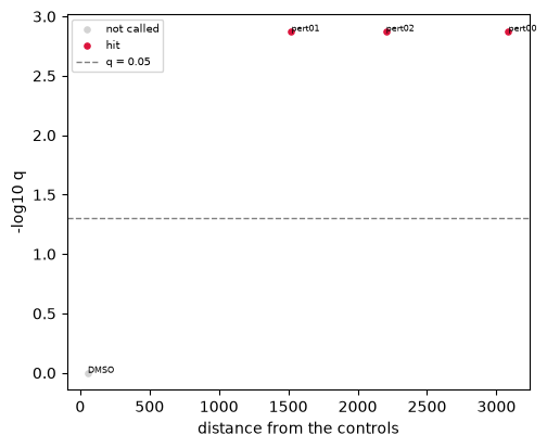
The controls are not called, which is the calibration check: DMSO scored against DMSO should get a high q-value, and it does. Every treated group is called.

Read the warning above. hit_calling splits the control wells, using half to fit the covariance and half to form the null, so 48 control wells leave 24 rows to estimate a 25×25 covariance. That is underdetermined, and the Mahalanobis distances depend more on the regularization than on the data. The ordering here is still correct, but on a real screen follow the warning: reduce the features first, or score a PCA representation with use_rep="X_pca". Tutorial 0 does the latter, which is why it shows no warning.

When the median hides the effect

method="mahalanobis" takes the median distance of a group’s rows from the control center. That is robust, but it misses a response in part of the population: if a fifth of the cells move a long way, the median of the whole group barely changes.

method="ks" compares the whole distribution of distances instead. The next cell builds this case: a plate with no injected effect, where 20% of one perturbation’s cells are shifted strongly.

partial = mt.ds.synthetic_plate(n_wells=96, n_cells=40, n_features=25, n_perturbations=2, effect_size=0.0, seed=0)
mt.pp.normalize(partial, by="Metadata_Plate", reference="negcon")

rng = np.random.default_rng(0)
target = np.flatnonzero((partial.obs["Metadata_Perturbation"] == "pert00").to_numpy())
responders = rng.choice(target, size=int(0.2 * target.size), replace=False)
values = partial.X.copy()
values[responders] += 8.0
partial.X = values

for method in ("mahalanobis", "ks"):
    mt.tl.hit_calling(partial, method=method, n_permutations=1000, key_added=method)
mt.tl.edistance(partial, n_permutations=500)

summary = {}
for name in ("mahalanobis", "ks", "edistance"):
    table = partial.uns["mantispy"][name].set_index("group")
    distance = table["distance"]
    summary[name] = {
        "pert00 (20% respond)": round(float(distance["pert00"]), 3),
        "pert01 (nothing)": round(float(distance["pert01"]), 3),
        "pert00 / pert01": round(float(distance["pert00"]) / max(abs(float(distance["pert01"])), 1e-9), 2),
        "pert01 called?": bool(table.loc["pert01", "is_hit"]),
    }
summary

{'mahalanobis': {'pert00 (20% respond)': 5.259,
  'pert01 (nothing)': 5.064,
  'pert00 / pert01': 1.04,
  'pert01 called?': False},
 'ks': {'pert00 (20% respond)': 0.205,
  'pert01 (nothing)': 0.037,
  'pert00 / pert01': 5.6,
  'pert01 called?': False},
 'edistance': {'pert00 (20% respond)': 2.668,
  'pert01 (nothing)': 0.004,
  'pert00 / pert01': 657.02,
  'pert01 called?': True}}

The median Mahalanobis distance separates the responder from the unchanged group by four percent. The KS statistic separates them more than fivefold, and the energy distance, which compares the whole distributions, by orders of magnitude. This is the reason to keep single cells: after aggregation, the 20% is averaged into the 80%.

The q-values need care here, and the three methods differ. Mahalanobis and KS both leave pert01 uncalled, which is correct because nothing was done to it. For Mahalanobis this is not evidence of good calibration: pert00 and pert01 sit at a distance ratio of 1.04, so it barely separated the two groups in either direction, and the uncalled pert01 reflects low sensitivity more than a correct rejection. edistance calls pert01, at a distance of 0.004 against 2.67 for pert00: more than six hundred times smaller, and still significant.

The energy distance works as designed here. With a thousand cells per group, its permutation null is tight enough that almost any difference is significant, and at cell resolution almost any two groups differ. Rank by the statistic and use the q-value to discard, not to order. Check a method’s calibration on your own screen with mt.metrics.diagnose_testing instead of assuming it because the method reports a q-value.

Which features moved

tl.effect_size gives Cohen’s d, or a robust z with method="robust_z", for every feature and every group, with a Mann-Whitney p-value and a Benjamini-Hochberg q-value. The simulation injected its effect into five features per perturbation, so the check is whether those five come out on top.

mt.tl.effect_size(wells)
table = wells.uns["mantispy"]["effect"]
truth = wells.uns["mantispy"]["truth"]["affected_features"]

ranking = {}
for group, injected in truth.items():
    if not injected:
        continue
    ordered = list(
        table[table["group"] == group].set_index("feature")["effect"].abs().sort_values(ascending=False).index
    )
    ranking[group] = sorted(ordered.index(name) + 1 for name in injected)
{"features per group": wells.n_vars, "ranks of the injected features": ranking}

{'features per group': 25,
 'ranks of the injected features': {'pert00': [1, 2, 3, 4, 5],
  'pert01': [1, 2, 3, 4, 5],
  'pert02': [1, 2, 3, 4, 5]}}

ax = mt.pl.feature_volcano(wells, group="pert00")
plt.show()

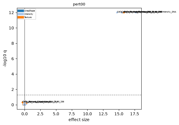
The five injected features take the top five places out of twenty-five in every group. The volcano plot colors each point by what the feature measures. That annotation comes from parsing the CellProfiler names (tutorial 1), so nothing had to be supplied here.

A change in shape

An effect size compares locations. A perturbation that widens a feature’s distribution without moving its center has an effect size of zero, but it is still a biological change: some cells reacted and others did not.

tl.wasserstein_features compares the distributions themselves.

spread = wells.copy()
values = spread.X.copy()
selected = (spread.obs["Metadata_Perturbation"] == "pert01").to_numpy()
values[selected, 0] = rng.standard_normal(int(selected.sum())) * 5.0
spread.X = values

mt.tl.effect_size(spread)
mt.tl.wasserstein_features(spread)

position = spread.uns["mantispy"]["effect_groups"].index("pert01")
{
    "feature": str(spread.var_names[0]),
    "cohen's d": round(float(spread.varm["effect"][0, position]), 3),
    "wasserstein": round(float(spread.varm["wasserstein"][0, position]), 3),
}

{'feature': 'Cells_AreaShape_Area', "cohen's d": -0.296, 'wasserstein': 4.008}

Cohen’s d is 0.3, a small effect by any convention, and it is that large only because pert01’s median already differed slightly from the control median. The Wasserstein distance is thirteen times larger. Ranked by effect size, this feature does not stand out; ranked by distributional distance, it is first.

One profile per perturbation

tl.consensus collapses replicates into one signature per perturbation. The default, modz, weights each replicate by how well it agrees with the others, so a single bad well is down-weighted instead of averaged in.

modz is a weighted mean. It beats the plain mean by a wide margin but does not beat the median. On BBBC021, not-same-compound MOA retrieval is 0.777 with method="median" and 0.660 with modz. Compare both on your own data.

signatures = mt.tl.consensus(wells, method="modz")
weights = signatures.uns["mantispy"]["consensus_weights"]
{
    "signatures": signatures.shape,
    "resolution": signatures.uns["mantispy"]["resolution"],
    "weights sum to one per group": bool(np.allclose(weights.groupby("group")["weight"].sum(), 1.0, atol=1e-3)),
}

{'signatures': (4, 25),
 'resolution': 'perturbation',
 'weights sum to one per group': True}

Dose response

With a concentration series, the question becomes whether the effect grows with dose. An active compound gives a monotonic trend and a sigmoid curve; a well-position artifact does not.

tl.dose_response reports a Spearman trend for every compound, which assumes nothing about the curve’s shape, and fits a four-parameter logistic for an EC50 wherever there are at least min_doses distinct doses. The minimum exists because four parameters fitted to three points give a number without support.

from mantispy.tl._dose import four_parameter_logistic

dosed = wells.copy()
n = dosed.n_obs
dose = np.tile([0.01, 0.1, 1.0, 10.0, 100.0], n)[:n]
compound = rng.permutation(np.where(np.arange(n) % 2 == 0, "active", "flat"))
dosed.obs["Metadata_Compound"] = compound
dosed.obs["Metadata_Concentration"] = dose

true_ec50 = 1.0
response = np.where(
    compound == "active",
    four_parameter_logistic(np.log10(dose), 0.0, 10.0, np.log10(true_ec50), 1.5),
    0.0,
)
dosed.obs["hits_distance"] = response + rng.normal(0, 0.2, n)

mt.tl.dose_response(dosed)
dosed.uns["mantispy"]["dose_response"].round(3)

	compound	n_doses	spearman	pvalue	ec50	hill_slope	bottom	top	r_squared	fit_ok	qvalue
0	active	5	0.939	0.000	0.992	1.537	0.023	9.941	0.998	True	0.000
1	flat	5	-0.130	0.207	113.598	6.754	0.020	-0.265	0.043	False	0.207

ax = mt.pl.dose_response(dosed, compound="active")
plt.show()

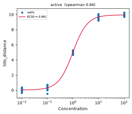
The fitted EC50 matches the concentration the curve was built with, and the compound with no dose dependence has no trend.

The flat compound’s row is also worth reading. The optimizer converged on it and reports an EC50 of 113.6 and a Hill slope of 6.8, which look like a result on their own. Four parameters fitted to five points converge on almost anything: on pure noise at six doses the optimizer succeeds 59 times in 60.

r_squared and fit_ok catch this. The curve explains 4% of the flat compound’s variance against 99.8% for the active one, and its EC50 lies outside the tested doses, so it is an extrapolation. fit_ok requires both a good fit and an EC50 inside the tested range, so the flat row fails. Check the Spearman trend and its q-value first in any case: a monotonic trend assumes nothing about shape and works with three points, where an EC50 fit does not.

What is on the object now

Every result is stored on the object, so mt.io.write saves all of it and a later session can continue from here.

what	where
hit table	uns["mantispy"]["hits"]
per-row distance and q	obs["hits_distance"], obs["hits_qvalue"]
effect sizes	varm["effect"] and uns["mantispy"]["effect"]
Wasserstein distances	varm["wasserstein"] and uns["mantispy"]["wasserstein"]
e-distances	uns["mantispy"]["edistance"]
dose response	uns["mantispy"]["dose_response"]
replicate weights	uns["mantispy"]["consensus_weights"] on the consensus object

Next: mechanism of action, on real data.